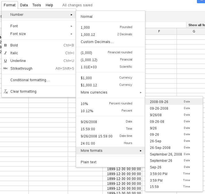
I was unsatisfied by the available date time formats in Google Docs Spreadsheets:
You only have one format for both date and time. By the way, the menus name Number is not really a proper one, although everything can actually boil down to just two numbers. Still, bizarre to me.
An example to show you why I was unhappy, and its the final spreadsheet as well:
See the Column A, it looks so ugly, the dates are not aligned. As a programmer, Id prefer every part is prefixed with zero when needed, or align well at least. Unfortunately, there is no options for you to change the output format, you have to stick with it if you can only do button-clicking. However, if you can do more than that, then TEXT() function is the way to code. (laughter, I found that its strange to use that word with Spreadsheet)
The syntax is:
TEXT(number, format)
Here, number is the date time and format is similar to the letters from the arguments of strftime in other languages. (laughter, again) Google really does a terrible job on documenting for products like Spreadsheets, end-user products but with coding aspect involving, I cant find any information about the format on this functions list. I really wonder who wrote that poor quality page. Same thing also happens on Google Analytics, its help about regular expression for filter is written poorly and many details are missing, I suspect those were written by whom dont know much about regular expressions. They try to write for people who dont have the background of programming, which is fine and makes perfect sense. The problem is the pages dont read so and the writers obviously dont have the background, either.
Anyway, you can find the format in this spreadsheet via (Unofficial) Google Spreadsheets FAQ.
As you can see in Column B, it shows what I like. The formula I use is:
ARRAYFORMULA(TEXT(FILTER(A2:A, NOT(ISBLANK(A2:A))), "YYYY-MM-dd HH:mm:ss"))
Its little complicated, perhaps scary if you dont know much about programming. Actually, if you do, then its even more scarier for you than for people who dont have coding knowledge. That formula read not much sense when I firstly made it work. I still didnt know how I managed to guess the correct way to code after read Spreadsheets help page.
Because I dont want to manually expand the cell to fill in formula, therefore this must be utilized. It is a great way to let code do tedious tasks for you, dragging bottom-right square to automatically fill in. See? Exclamation the cell index increases one its own. Well, thats for noob or people have 24 hours and 1 second a day, you clearly have no idea what magic really is.
ARRAYFORMULA() is the one with the magic, you feed it with an array, it results in the same dimension of array after processing with the formula. In this case, they are TEXT() and functions within. You can see I also use FILTER() to filter out blank cells, if you skip filtering, then it results like Column E. FILTER will only output the element when the value is true from the same index of array in the second argument NOT(ISBLANK(A2:A)). A2:A is an array starting with Cell A2, then Cell A3, , to the rest of Column A. With all these, the output is clean and job is done.
The drawback with this method is you need to have two columns for same data, thats what you need to accept. If the spreadsheet doesnt have high volume of editing, then you can just hide the raw date time column and only unhide when you need to add new row of data. There is another way to deal with this issue if its one for you, use two columns for date and time, separately. But you may need to use two columns at the same time when something needs the date time information.
By the way, Google Docs Spreadsheets needs to have paired parenthesis highlighting, I can already lose in this formula and this is not the most complicated one that I have ever written. About two weeks ago, I made this form for favorite Unix commands poll, had to spend some time to count how many parenthesis I had opened and closed.
